DuckDB

Note

JupySQL also supports DuckDB with a native connection (no SQLAlchemy needed), to learn more, see the tutorial. To learn the differences, click here.

JupySQL integrates with DuckDB so you can run SQL queries in a Jupyter notebook. Jump into any section to learn more!

Pre-requisites for .csv file

%pip install jupysql duckdb duckdb-engine --quiet
%load_ext sql
%sql duckdb://

Note: you may need to restart the kernel to use updated packages.

Connecting to 'duckdb://'

Load sample data

Get a sample .csv file:

from urllib.request import urlretrieve

_ = urlretrieve(
    "https://raw.githubusercontent.com/mwaskom/seaborn-data/master/penguins.csv",
    "penguins.csv",
)

Query

The data from the .csv file must first be registered as a table in order for the table to be listed.

%%sql
CREATE TABLE penguins AS SELECT * FROM penguins.csv

Running query in 'duckdb://'

Count

The cell above allows the data to now be listed as a table from the following code:

%sqlcmd tables

Name
penguins

List columns in the penguins table:

%sqlcmd columns -t penguins

name	type	nullable	default	autoincrement	comment
species	VARCHAR	True	None	False	None
island	VARCHAR	True	None	False	None
bill_length_mm	DOUBLE PRECISION	True	None	False	None
bill_depth_mm	DOUBLE PRECISION	True	None	False	None
flipper_length_mm	BIGINT	True	None	False	None
body_mass_g	BIGINT	True	None	False	None
sex	VARCHAR	True	None	False	None

%%sql
SELECT *
FROM penguins.csv
LIMIT 3

Running query in 'duckdb://'

species	island	bill_length_mm	bill_depth_mm	flipper_length_mm	body_mass_g	sex
Adelie	Torgersen	39.1	18.7	181	3750	MALE
Adelie	Torgersen	39.5	17.4	186	3800	FEMALE
Adelie	Torgersen	40.3	18.0	195	3250	FEMALE

%%sql
SELECT species, COUNT(*) AS count
FROM penguins.csv
GROUP BY species
ORDER BY count DESC

Running query in 'duckdb://'

species	count
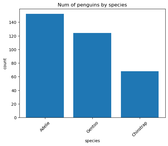
Adelie	152
Gentoo	124
Chinstrap	68

Plotting

%%sql species_count <<
SELECT species, COUNT(*) AS count
FROM penguins.csv
GROUP BY species
ORDER BY count DESC

Running query in 'duckdb://'

ax = species_count.bar()
# customize plot (this is a matplotlib Axes object)
_ = ax.set_title("Num of penguins by species")

/home/docs/checkouts/readthedocs.org/user_builds/jupysql/checkouts/938/src/sql/run/resultset.py:371: UserWarning: .bar() is deprecated and will be removed in a future version. Use %sqlplot bar instead. For more help, find us at https://ploomber.io/community 
  warnings.warn(

Pre-requisites for .parquet file

%pip install jupysql duckdb duckdb-engine pyarrow --quiet
%load_ext sql
%sql duckdb://

Note: you may need to restart the kernel to use updated packages.
The sql extension is already loaded. To reload it, use:
  %reload_ext sql

Load sample data

Get a sample .parquet file:

from urllib.request import urlretrieve

_ = urlretrieve(
    "https://d37ci6vzurychx.cloudfront.net/trip-data/yellow_tripdata_2021-01.parquet",
    "yellow_tripdata_2021-01.parquet",
)

Query

Identically, to list the data from a .parquet file as a table, the data must first be registered as a table.

%%sql
CREATE TABLE tripdata AS SELECT * FROM "yellow_tripdata_2021-01.parquet"

Running query in 'duckdb://'

Count

The data is now able to be listed as a table from the following code:

%sqlcmd tables

Name
tripdata
penguins

List columns in the tripdata table:

%sqlcmd columns -t tripdata

name	type	nullable	default	autoincrement	comment
VendorID	BIGINT	True	None	False	None
tpep_pickup_datetime	TIMESTAMP	True	None	False	None
tpep_dropoff_datetime	TIMESTAMP	True	None	False	None
passenger_count	DOUBLE PRECISION	True	None	False	None
trip_distance	DOUBLE PRECISION	True	None	False	None
RatecodeID	DOUBLE PRECISION	True	None	False	None
store_and_fwd_flag	VARCHAR	True	None	False	None
PULocationID	BIGINT	True	None	False	None
DOLocationID	BIGINT	True	None	False	None
payment_type	BIGINT	True	None	False	None
fare_amount	DOUBLE PRECISION	True	None	False	None
extra	DOUBLE PRECISION	True	None	False	None
mta_tax	DOUBLE PRECISION	True	None	False	None
tip_amount	DOUBLE PRECISION	True	None	False	None
tolls_amount	DOUBLE PRECISION	True	None	False	None
improvement_surcharge	DOUBLE PRECISION	True	None	False	None
total_amount	DOUBLE PRECISION	True	None	False	None
congestion_surcharge	DOUBLE PRECISION	True	None	False	None
airport_fee	DOUBLE PRECISION	True	None	False	None

%%sql
SELECT tpep_pickup_datetime, tpep_dropoff_datetime, passenger_count
FROM "yellow_tripdata_2021-01.parquet"
LIMIT 3

Running query in 'duckdb://'

tpep_pickup_datetime	tpep_dropoff_datetime	passenger_count
2021-01-01 00:30:10	2021-01-01 00:36:12	1.0
2021-01-01 00:51:20	2021-01-01 00:52:19	1.0
2021-01-01 00:43:30	2021-01-01 01:11:06	1.0

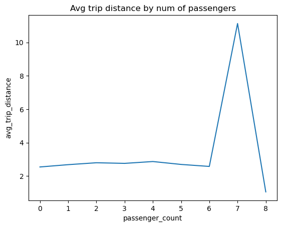
%%sql
SELECT
    passenger_count, AVG(trip_distance) AS avg_trip_distance
FROM "yellow_tripdata_2021-01.parquet"
GROUP BY passenger_count
ORDER BY passenger_count ASC

Running query in 'duckdb://'

passenger_count	avg_trip_distance
0.0	2.5424466811344635
1.0	2.6805563237139625
2.0	2.7948325921160815
3.0	2.757641060657793
4.0	2.8681984015618216
5.0	2.6940995207307994
6.0	2.5745177825092593
7.0	11.134
8.0	1.05
None	29.665125772734566

Truncated to displaylimit of 10.

Plotting

%%sql avg_trip_distance <<
SELECT
    passenger_count, AVG(trip_distance) AS avg_trip_distance
FROM "yellow_tripdata_2021-01.parquet"
GROUP BY passenger_count
ORDER BY passenger_count ASC

Running query in 'duckdb://'

ax = avg_trip_distance.plot()
# customize plot (this is a matplotlib Axes object)
_ = ax.set_title("Avg trip distance by num of passengers")

/home/docs/checkouts/readthedocs.org/user_builds/jupysql/checkouts/938/src/sql/run/resultset.py:322: UserWarning: .plot() is deprecated and will be removed in a future version. For more help, find us at https://ploomber.io/community 
  warnings.warn(

Plotting large datasets

New in version 0.5.2.

This section demonstrates how we can efficiently plot large datasets with DuckDB and JupySQL without blowing up our machine’s memory. %sqlplot performs all aggregations in DuckDB.

Let’s install the required package:

%pip install jupysql duckdb duckdb-engine pyarrow --quiet

Note: you may need to restart the kernel to use updated packages.

Now, we download a sample data: NYC Taxi data split in 3 parquet files:

from pathlib import Path
from urllib.request import urlretrieve

N_MONTHS = 3

# https://www1.nyc.gov/site/tlc/about/tlc-trip-record-data.page
for i in range(1, N_MONTHS + 1):
    filename = f"yellow_tripdata_2021-{str(i).zfill(2)}.parquet"
    if not Path(filename).is_file():
        print(f"Downloading: {filename}")
        url = f"https://d37ci6vzurychx.cloudfront.net/trip-data/{filename}"
        urlretrieve(url, filename)

Downloading: yellow_tripdata_2021-02.parquet

Downloading: yellow_tripdata_2021-03.parquet

In total, this contains more then 4.6M observations:

%%sql
SELECT count(*) FROM 'yellow_tripdata_2021-*.parquet'

Running query in 'duckdb://'

count_star()
4666630

Let’s use JupySQL to get a histogram of trip_distance across all 12 files:

%sqlplot histogram --table yellow_tripdata_2021-*.parquet --column trip_distance --bins 50

<Axes: title={'center': "'trip_distance' from 'yellow_tripdata_2021-*.parquet'"}, xlabel='trip_distance', ylabel='Count'>

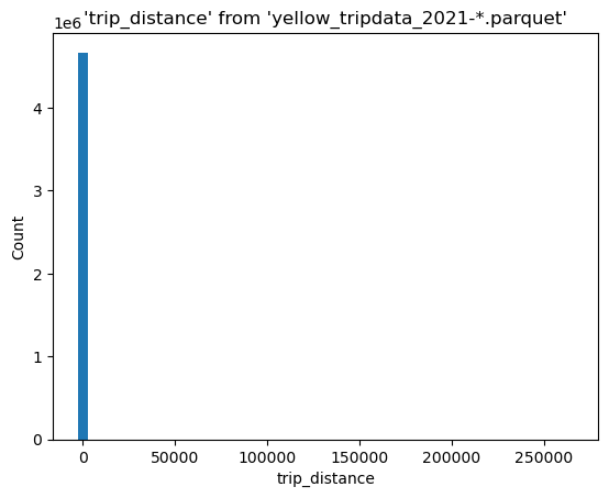
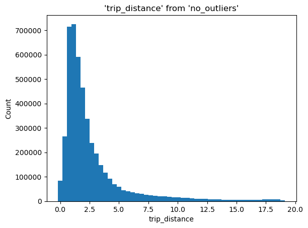
We have some outliers, let’s find the 99th percentile:

%%sql
SELECT percentile_disc(0.99) WITHIN GROUP (ORDER BY trip_distance)
FROM 'yellow_tripdata_2021-*.parquet'

Running query in 'duckdb://'

quantile_disc(0.99 ORDER BY trip_distance)
18.93

We now write a query to remove everything above that number:

%%sql --save no_outliers --no-execute
SELECT trip_distance
FROM 'yellow_tripdata_2021-*.parquet'
WHERE trip_distance < 18.93

Running query in 'duckdb://'

Skipping execution...

%sqlplot histogram --table no_outliers --column trip_distance --bins 50

<Axes: title={'center': "'trip_distance' from 'no_outliers'"}, xlabel='trip_distance', ylabel='Count'>

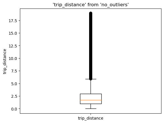
%sqlplot boxplot --table no_outliers --column trip_distance

<Axes: title={'center': "'trip_distance' from 'no_outliers'"}, ylabel='trip_distance'>

Querying existing dataframes

import pandas as pd
from sqlalchemy import create_engine

engine = create_engine("duckdb:///:memory:")
df = pd.DataFrame({"x": range(100)})

%sql engine

%%sql
SELECT *
FROM df
WHERE x > 95

Running query in 'duckdb:///:memory:'

x
96
97
98
99

Passing parameters to connection

from sqlalchemy import create_engine

some_engine = create_engine(
    "duckdb:///:memory:",
    connect_args={
        "preload_extensions": [],
    },
)

%sql some_engine